Article

In-Season Interactions between Vine Vigor, Water Status and Wine Quality in Terrain-Based Management-Zones in a ‘Cabernet Sauvignon’ Vineyard

1
The Robert H. Smith Institute of Plant Sciences and Genetics in Agriculture, The Robert H. Smith Faculty of Agriculture, Food & Environment, The Hebrew University of Jerusalem, Rehovot 76100, Israel
2
Agricultural Engineering, Agricultural Research Organization—Volcani Institute, P.O. Box 15159, Rishon LeZion 7505101, Israel
3
Department of Chemical Engineering, Ariel University, Ariel 40700, Israel
4
Eastern R & D Center, Department of Agriculture and Oenology, Ariel 40700, Israel
5
TerraVision Lab, Midreshet Ben-Gurion 8499000, Israel
6
Independent Researcher, Variability, Ashalim 85512, Israel
7
Gilat Research Center, Soil, Water and Environmental Sciences, Agricultural Research Organization—Volcani Institute, Mobile Post Negev 2 85280, Israel
*
Author to whom correspondence should be addressed.
Remote Sens. 2021, 13(9), 1636; https://doi.org/10.3390/rs13091636
Submission received: 21 March 2021 / Revised: 17 April 2021 / Accepted: 19 April 2021 / Published: 22 April 2021

Abstract

:
Wine quality is the final outcome of the interactions within a vineyard between meteorological conditions, terrain and soil properties, plant physiology and numerous viticultural decisions, all of which are commonly summarized as the terroir effect. Associations between wine quality and a single soil or topographic factor are usually weak, but little information is available on the effect of terrain (elevation, aspect and slope) as a compound micro-terroir factor. We used the topographic wetness index (TWI) as a steady-state hydrologic and integrative measure to delineate management zones (MZs) within a vineyard and to study the interactions between vine vigor, water status and grape and wine quality. The study was conducted in a commercial 2.5-ha Vitis vinifera ‘Cabernet Sauvignon’ vineyard in Israel. Based on the TWI, the vineyard was divided into three MZs located along an elongate wadi that crosses the vineyard and bears water only in the rainy winter season. MZ1 was the most distant from the wadi and had low TWI values, MZ3 was closest to the wadi and had high TWI values. Remotely sensed crop water stress index (CWSI) was measured simultaneously with canopy cover (as determined by normalized difference vegetation index; NDVI) and with field measurements of midday stem water potential (Ψstem) and leaf area index (LAI) on several days during the growing seasons of 2017 and 2018. Vines in MZ1 had narrow trunk diameter and low LAI and canopy cover on most measurement days compared to the other two MZs. MZ1 vines also exhibited the highest water stress (highest CWSI and lowest Ψstem), lowest yield and highest wine quality. MZ3 vines showed higher LAI on most measurement days, lowest water deficit stress (Ψstem) during phenological stage I, highest yield and lowest wine quality. Yet, in stage III, MZ3 vines exhibited a similar water deficit stress (CWSI and Ψstem) as MZ2, suggesting that the relatively high vigor in MZ3 vines resulted in higher water deficit stress than expected towards the end of the season, possibly because of high water consumption over the course of the season. TWI and its classification into three MZs served as a reliable predictor for most of the attributes in the vineyard and for their dynamics within the season, and, thus, can be used as a key factor in delineation of MZs for irrigation. Yet, in-season remotely sensed monitoring is required to follow the vine dynamics to improve precision irrigation decisions.

1. Introduction

Spatial variability in terrain (elevation, slope and aspect) and soil properties (texture and depth) can lead to different extents of soil water availability even within a small vineyard [1]. Therefore, genetically identical vines of the same age differ in vine growth and vigor and in vine physiological parameters. The accumulated effect over the years can lead to high variation in grape yield and fruit maturity. As variability increases, irrigation efficiency decreases, such that the full potential of the vineyard cannot be achieved [2]. Precision irrigation through irrigation management zones (IMZs) strategy aims at targeting this challenge. Generally, delineation of MZs is a way of classifying the spatial variability within a field [3]. In the context of irrigation, a MZ is a subregion of a field that is (relatively) homogeneous in its water availability for which a single rate of irrigation is appropriate.
In semiarid areas, soil hydraulic and physical properties often control vine water status [4], and therefore can be used to delineate IMZs. Among those properties, maps of apparent soil electrical conductivity (ECa) have been extensively used to delineate MZs in vineyards [5,6]. Elevation, slope, soil texture and soil depth have also been utilized for MZ delineation in vineyards [7,8,9]. It has been shown in previous studies that topographic inclination and slope can be key factors affecting soil and vine water dynamics [10,11]. Topographic wetness index (TWI), a steady-state hydrologic variable, mainly determined by slope, can be a good parameter for IMZ as it provides an estimate of the water drainage dynamics within the field during the winter and thus affects vine water availability during the spring and summer [12]. In recent studies, TWI was used for flood risk assessment [13] and as an additional variable for IMZ delineation in vineyards [9,14].
Stem water potential (Ψstem) is a sensitive indicator for vine water status [15] and should be frequently monitored when used to drive irrigation management [16,17,18]. Enhancing fruit quality for red wine production necessitates accurate control of the water deficit during the growing season [19]. For instance, grape berry development can be inhibited by temporary water deficit during stage I (anthesis-bunch closure), thus inducing a high skin-to-pulp ratio [16]. Since most of the fruit color and phenolic and aromatic components are concentrated in the skins, higher skin-to-pulp ratio in the grape must is desirable [20]. In addition, it was shown that water deficit during stage III (veraison-harvest) also promotes high concentrations of anthocyanins in red wine grapes and their wines [21]. However, severe water deficit stress resulted in negative effects on a vineyard’s endurance because of structural damage to the xylem and deterioration of the hydraulic system of the vine [17].
In order to adopt best irrigation practices in a vineyard, an IMZ strategy should include frequent monitoring of vine water status to drive appropriate local irrigation management [2]. Yet, while on the scale of the entire vineyard Ψstem can be measured in a few representative vines, MZ-based irrigation requires additional laborious and time-consuming measurements to represent the water status in each IMZ. Aerial thermal-imaging could serve as an alternative way of assessing the spatial variability of water status in the vineyard. In previous studies, ground based, proximal and airborne thermal imagery was used for irrigation scheduling [22] or for water status assessment [23,24,25] in vineyards. Thermal imaging was also used to estimate in-field spatial variability of water deficit stress [26] and to classify a vineyard into IMZs [14].
Delineation of IMZs using geomorphological data of soil texture and topography [27,28] is based on the assumption that IMZs are static. Each IMZ is characterized by a different level of water availability, and differences between IMZs are assumed to be stable throughout the season. Further, it is generally assumed that vine water status is positively correlated with soil water availability. Accordingly, in IMZs with high water availability vines would grow more canopy and would not suffer from water shortage, while in IMZs with low water availability vines would suffer from water deficit stress and grow a smaller canopy. However, recent studies have indicated that the relationships between soil water availability and plant water status is complicated. For example, vines with higher water availability and LAI at the beginning of season were found to reach higher water deficit stress at the end of the season because of wider vessels and increased specific hydraulic conductivity [17,29] or greater leaf area [26].
The objective of this study was to characterize the seasonal dynamics of vine vigor and water deficit stress in TWI-based MZs and to assess its effects on fruit yield, fruit quality and wine quality. The study demonstrates the role of aerial remote sensing in mapping the variability of vine vigor and water status required for a MZ-based irrigation strategy.

2. Materials and Methods

2.1. Study Site

The study was conducted in a commercial vineyard of Vitis vinifera L. ‘Cabernet Sauvignon’ grafted onto 101-14 rootstock in Mevo-Beitar, Israel (31°43′N; 35°06′E; Figure 1). Vine spacing was 1.5 m within rows and 3 m between rows (2222 vines per hectare), and the vineyard consisted of 5522 vines. The vines were planted in 2011, with a row direction of 117–297°, and were trained to a vertical shoot positioned trellis system with two foliage wires on each side. The elevation of the vineyard varied from 672 to 702 m above sea level (Table 1), with the eastern part reaching higher elevation and gradually declining towards the west. The area’s lithology is dominated by limestone, frequently mixed with chalk and marl, and covered with shallow terra-rosa soil. During the 2017-2018 growing seasons, the vineyard was drip-irrigated using a computer-controlled system (Dream 1, Talgil, Israel) with one drip line (16 mm) per row at 1.6 L/h in-line, pressure-compensated drippers spaced 0.75 m apart (Uni-Ram, Netafim, Israel). Irrigation was based on crop coefficients and potential evapotranspiration, calculated according to the ASCE Penman-Monteith equation [30]. At all fruit development stages, the basic crop coefficient was 0.2. Ψstem measurements were used to correct the irrigation factor as described at Bahat et al., [31].
The vineyard was delineated into 20 management cells (MCs; referred by the letters A–T) and 6 vines per MC (120 vines in total) were selected as measurement vines (Figure 1).
In 2017, irrigation was uniform for the entire vineyard and reached 98 mm for the season. In 2018 a drip precision irrigation system was installed in the western block (MCs A–J). In that season, the vineyard was irrigated with a total of 32 mm on average, with most of the western MCs receiving within ±5 mm of the average. The exception to this being MC C, which was irrigated with 66 mm, which had no impact on this study’s results [31]. More detail of the site and experiment can be found at the project story map website [32].

2.2. Terrain and Soil Measurements

The spatial variability of soil and terrain was mapped and quantified by various field attributes (Figure 2a–d, Table 1). A contour digital elevation model (DEM) with spatial resolution of 1 m was created based on a local elevation survey using real time kinematic global positioning system (RTK). The DEM was further used to create topographic layers using the ‘Topo to Raster’ tool in ArcMap 10.6 (ESRI Inc. Redlands, CA, USA), including elevation (Figure 2a) and slope, and was further analyzed to create the TWI layer (Figure 2b). TWI was originally proposed by Beven and Kirkby [33] and provides a relative, not absolute, measure of the soil moisture status of each pixel in a defined area. The index was calculated using the “dynatopmodel” package in R [34] by the equation:
T W I = ln ( A t a n β )
where A is the specific area, or the upstream contributing area (m2) for each pixel, and β is the local slope in the steepest down slope direction in degrees.
Apparent electrical conductivity (ECa) was determined on 10 April 2018 by a four-probe soil resistance sensor (Soil EC 3100; Veris Technologies, Salina, KS) at field capacity as recommended by the protocol for conducting a field-scale ECa survey [35]. Data from the shallow layer (0–75 cm) were utilized for this study as it represents the vast majority of expected grapevine active root zone [36]. An ECa map (Figure 2d) was created from 4037 points recorded using the geostatistical module contained in ArcMap 10.6, interpolated according to the inverse distance weighting (IDW) method.
Soil depth levels were measured using an 80 cm diameter hydraulic earth auger connected to a small tractor at 81 randomly selected points defined using stratified random sampling. The exact depth was recorded when the auger reached bedrock. A soil depth map (Figure 2c) was created using the geostatistical module contained in ArcMap 10.6, interpolated according to the IDW method.

2.3. Plant Vigor Measurements

2.3.1. Ground Measurements

LAI of the 120 measurement vines was determined during the growing season using a canopy analysis system (SunScan model SS1-R3-BF3; Delta-T Devices, Cambridge, UK). The system was operated using the standard protocol recommended by the manufacturer, and all measurements were conducted while the zenith angle was below 30°. The LAI values obtained were compared with measurements following destructive defoliation of leaves from 39 vines (3 cultivars from 6 sites), using an area meter (model 3100; Li-Cor, Lincoln, Nebraska). The two measurement methods were found to have strong linear relationship [37]. Trunk diameter was measured during January 2017 using digital calipers (075430, Signet, Taiwan) for all vines (n = 5522), at a height of 50 cm above ground, representing the cumulated multi-year vine vigor.

2.3.2. Remote-Sensing

Canopy cover was determined as the covered fraction (%) of NDVI within each MZ polygon. NDVI was calculated from a multispectral image of high spatial resolution (8 cm). The image was acquired between 11:45–12:00 Israel Standard Time by an airborne multispectral camera MicaSense RedEdge MX (MicaSense® Inc, Seattle, WA, USA). The RedEdge MX has five sensors (blue: 465–485 nm, green: 550–570 nm, red: 663–673 nm, red edge: 712–722 nm, and near infrared: 820–860 nm). It also has an external irradiance sensor with GPS and inertial measurement unit (IMU) placed on top of the UAV to capture sensor angle, sun angle, location, and irradiance for each image during flight. Red and near infrared (NIR) bands were used to calculate NDVI using the equation:
N D V I = ρ ( N I R ) ρ ( R e d ) ρ ( N I R ) + ρ ( R e d )
where ρ(NIR) is the reflectance value for near infrared band (center wavelength 0.84 µm) and ρ(Red) is the reflectance value for the visible red band (center wavelength 0.668 µm). NDVI values range between −1 and +1. Values below an empirical threshold of 0.3 were excluded as they mostly represented soil and weeds (Table 2).

2.4. Water Status Measurements

2.4.1. Ground Measurements

Midday stem water potential was measured around solar noon (12:00–14:30) on all measurement vines (n = 120). At four major phenological stages (Figure 3) we measured Ψstem on additional vines (extended measurement; n = 154) to allow for spatial interpolation using the kriging method (ArcMap 10.6). The measurements were conducted using pressure chambers (model Arimad 3000, MRC, Holon, Israel) according to the procedures of Boyer [38]. A mature, fully expanded, leaf from each measurement vine was bagged 2 h prior to acquisition with aluminum and plastic bags. The time elapsing between leaf excision and chamber pressurization was less than 20 s. Leaf stomatal conductance (gs) was measured on all measurement vines in the western block (n = 60) at three phenological stages during 2017, using a portable gas exchange measurement system (model LI-6400, Li-Cor) around solar noon (12:00–14:30). Further descriptive statistics can be found in Table 3.

2.4.2. Remote-Sensing

Crop water stress index (CWSI) based on canopy temperature [39] is widely used as a plant water stress indicator and as a tool for mapping in-field variability. Thermal imagery acquired at 11:45–12:00 from a UAV equipped with a FLIR SC655 thermal camera (FLIR® Systems, Inc., Bilerica, MA, USA) with 640 pixels × 480 pixels, sensitive in the spectral range of 7.5–13 µm and a measurement accuracy of ±0.5 °C was used to evaluate the vineyard’s canopy surface temperature. Image processing for pure canopy extraction included two major steps: 1. a temperature threshold of 45 °C was determined by a visual analysis of the temperature bimodal histogram to remove soil-associated pixels and 2. for masking other non-canopy pixels (mostly shade and grass), we used an NDVI image from the same campaign to indicate pixels with values above an empirical threshold of 0.3. Finally, the following equation was used as CWSI [39]:
CWSI = T c a n o p y T w e t T d r y T w e t
where Tcanopy is the temperature of the canopy, Twet is the temperature of a fully transpiring canopy and Tdry is the temperature of a non-transpiring canopy. Calculation of Tcanopy was done at the vine level—polygons of 80 cm × 140 cm for all 5522 vines were created, and the coolest 33% of the pixels within each of the polygons were averaged following Meron et al. [40]. Twet was calculated at the whole vineyard scale using the average temperature of the coolest 5% of the canopy pixels [41,42]. Tcanopy and Twet were calculated using the “raster” package in R [43]. For Tdry calculation, a portable meteorological station was positioned within the vineyard, which recorded the temperature during all hours of data collection at the canopy height by a data logger (Campbell Scientific, Logan, UT, USA). The average ambient air temperature during the flight was calculated. Tdry was calculated as Tair + 7 °C [41].

2.5. Yield and Fruit Quality Measurements

Yield was measured in two steps. First, hand-picked yield was determined at the vine scale. Twelve vines from each MC were selected, each vine was individually harvested and its total fruit weight and cluster number recorded, thus allowing calculation of cluster weight. Secondly, a mechanical grape harvester (New Holland, Braud 9040) with a continuous weighing system was used for spatial yield mapping at a resolution of 5 m. An interpolated thematic yield map (Figure 2e) was generated as described above (Section 2.2). Total soluble solids (TSSs) and fruit anthocyanin were determined for 104 geo-referenced sample sites within the vineyard that were collected a day before harvest. Twelve fruit clusters were collected at each sample site and were hand-crushed for fruit analysis using an automatic fruit must analyzer (SA-13, Maselli, Italy). Further descriptive statistics can be found in Table 4.

2.6. Wine Quality Assessments

The grapes of each MC (n = 20) were transported to Ariel winery and, after an over-night cooling, fruit must samples were taken for sugar content, pH and TA analyses. Wines were separately vinified using the following oenological technique: crushing and destemming; addition of SO2 (11 mg/Kg) and dry selected yeast (25 mg/Kg); 8-d fermentation at a controlled temperature in 100 L stainless steel tanks with three punches of the cap every day. Finally, the 20 wines were put in demijohns for malolactic fermentation and aging for 6 months. After bottling, the wines were tasted and evaluated by a test panel of 7–8 professional winemakers. The wine tasting was a “double-blind test,” with anonymous labels on the bottles of wines according to the ‘Organisation International de la Vigne et du Vin’ [44].

2.7. Vineyard Delineation to Management Zones

The relative influence of the three soil and terrain variables on vine water status was assessed using a predictive boosted trees model as a function of extended measurements of Ψstem at 4 different phenological stages. The boosted trees model produces an additive decision tree model that is based on many smaller decision trees that are constructed in layers. The tree in each layer consists of a small number of splits, typically five or fewer. Each layer is fit using the recursive fitting methodology [45]. Topographic wetness index and soil depth had the highest impact. At the beginning of the season, TWI had a higher impact on Ψstem variance implying that TWI better represents the soil water availability resulting from winter and spring precipitation. Therefore, TWI was selected as the basis for MZ delineation.
Delineation to MZs was determined using Iso Cluster unsupervised classification tool in ArcMap 10.6. The vineyard was delineated into 2, 3, 4 or 5 zones. Then, a single factor ANOVA was performed, and a goodness of variance fit (GVF) was calculated for each classification result of MZ, in order to minimize the member deviation from the class mean (within groups) while maximizing class mean deviation from other classes (between groups). The optimal number of MZs was determined when GVF reached a minimal threshold of 0.8, following Lowrance et al. [46].

2.8. Data Analysis

Analysis of variance (ANOVA) was performed to reveal differences between the different MZs within the vineyard (p < 0.05) for all variables with a normal distribution, and a multiple comparison test was done using the Tukey–Kramer HSD test. The non-parametric Steel–Dwass test was applied to determine differences between MZs for variables that were not normally distributed, namely gs, TSS and fruit must color. Statistical data analysis was performed using JMP software (Pro 15, SAS Institute, Cary, NC, USA) and R software [47].
In order to avoid spatial autocorrelation of CWSI, canopy cover, trunk diameter and yield variables, we selected 22 random points within a 6 m buffer in each MZ with a minimal distance of the calculated range of the semivariogram [48]. Random points were selected using the ‘Create Random Points’ Module, the semivariogram was calculated using the geostatistical wizard of ArcMap 10.6. Wine scores were classified for the MZs using Jenks natural breaks that minimizes each MZ’s average deviation from the MZ mean. All the analyses, interpolations and classification were calculated using ArcMap 10.6.

3. Results

3.1. Climate Conditions

The Judaean Hills region, where the study site was located, is characterized by a Mediterranean climate, with mean annual rainfall of 540 mm, typically concentrated between October and May [49]. Accumulated annual precipitation recorded at a meteorological station located 6 km from the vineyard was 369 and 452 mm/year for 2017 and 2018, respectively. The mean daily temperature ranged between 24.9 in August and 9.1 °C in January. Precipitation during the spring of 2016–2017 (between 1 March and 15 May) was low (17.2 mm) compared to the spring of 2018 (70.4 mm).

3.2. Geospatial Variables and Management Zones Delineation

TWI, which is affected mainly by the local slope (Equation 1), revealed a local wadi (Figure 2b, in blue) extending from east to west with a graduated effect around it. ECa and soil depth were characterized by a dispersed spatial pattern (Figure 2c,d). The relative influence of TWI, ECa and soil depth on vine water deficit stress (Ψstem) was analyzed on four phenological stages (Figure 4). On 23 May 2018 the relative influence of TWI on Ψstem was highest (76%), and therefore it was selected as the basis for the vineyard’s delineation into MZs (Figure 5).

3.3. Canopy Measurements

3.3.1. Ground Measurements

The seasonal trend of LAI showed higher canopy area in MZ3 on most of the measurement days during both growing seasons (Figure 6). The ANOVA results found a significant difference between MZ1 and MZ3 in 6 out of 9 days, and no differences between MZ2 and MZ3 (Table A1).
The average trunk diameter of the vines in MZ1 was 39.4 mm, which was significantly lower than the averaged trunk diameter in MZ2 (41.3 mm; Figure 7). MZ3 vine trunk diameter was intermediate (40.7 mm) and did not differ from those of MZ1 and MZ2.

3.3.2. Remote Sensing

The trend of canopy cover was relatively stable along the seasons, except for canopy trimming, which temporarily decreased canopy area for all MZ. On 8 out of 10 measurement days during the season, canopy cover in MZ1 was lower than canopy cover in at least one of the other 2 MZs (Figure 8).

3.4. Vine Water Status

3.4.1. Ground Measurements

The trend of Ψstem (Figure 9) exhibited low water deficit stress at the beginning of each season, gradually becoming higher towards harvest time. MZ1 had the greatest water deficit stress (lower Ψstem values) compared to MZ2 and MZ3 in most cases. MZ3 and MZ2 had a similar trend of Ψstem for all stages in both years, in 9 out of 18 measurements. MZ3 exhibited intermediate values between MZ1 to MZ2 and did not statistically differ from the other two MZs (Table A2). Stomatal conductance (gs) at the beginning of the 2017 season (20 June) was high and similar in all 3 MZs. On the other two measurement days gs was lower in MZ1 than in MZ2, with intermediate values for MZ3, suggesting a temporal change of MZ3 water status within the season (Figure 10).

3.4.2. Remote Sensing

Management zone (MZ) 1 demonstrated the highest water deficit stress, determined by higher CWSI values compared to MZ2 and MZ3 in most cases (Figure 11). In 2017, MZ3 and MZ2 had a similar trend of CWSI, while 2018 results demonstrated larger differences. At the beginning of the 2018 season (during stages I and II) MZ3 followed a similar trend as MZ2, but for the last three measurements of the season, it had higher values of CWSI.

3.5. Yield Components, Fruit and Wine Quality

MZ1 had the lowest yield, cluster weight and cluster number in 2017, and the highest TSS and fruit color (OD 420 + 520) in 2018. MZ2 and MZ3 exhibited similar responses regarding yield and its components, TSS, fruit must color and wine quality (Figure 12, Figure 13 and Figure 14).

4. Discussion

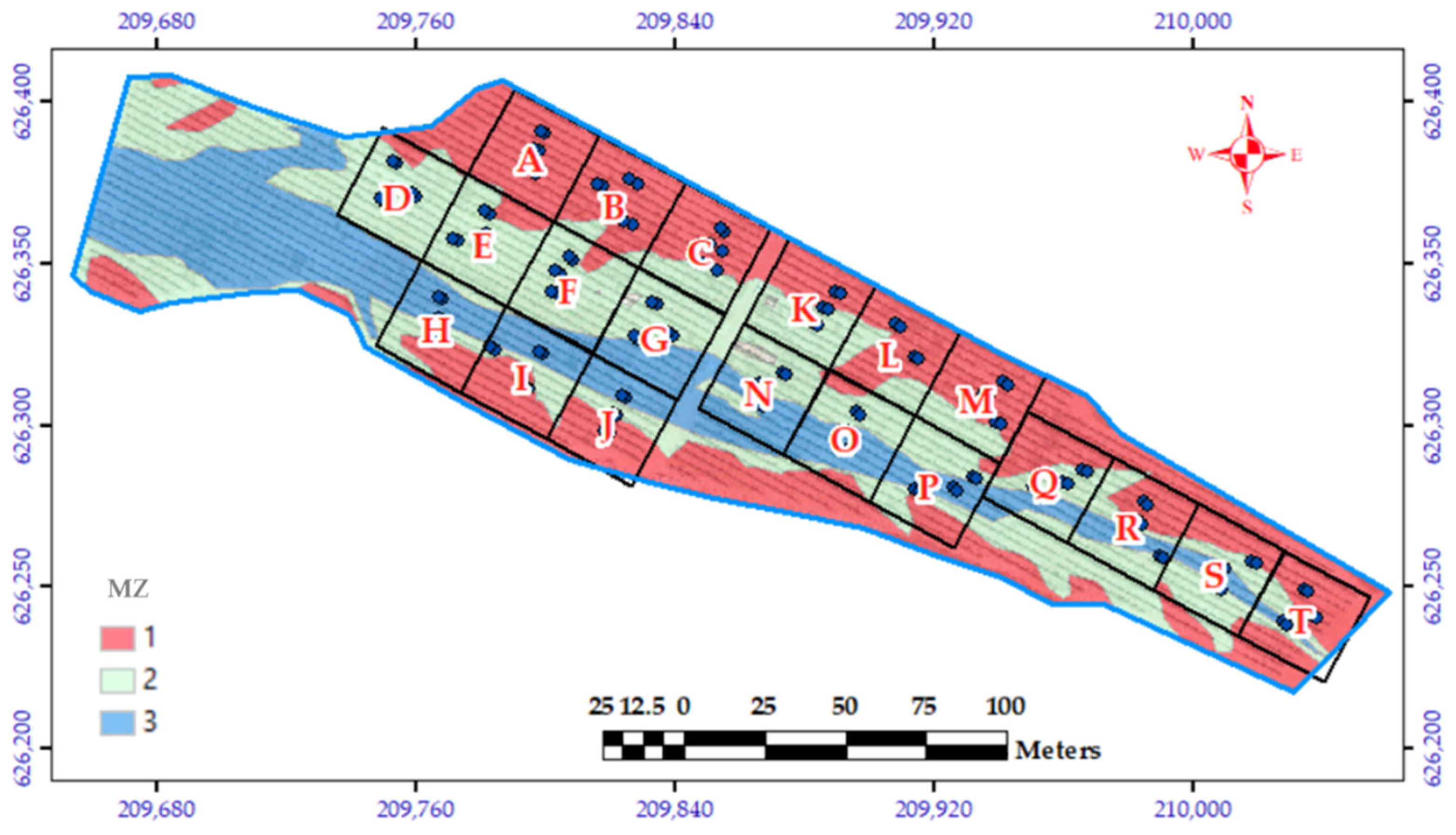
We defined and evaluated three MZs within a wine grape vineyard, based on a single topographic variable (TWI). Differences between MZs were continuously evaluated throughout two growing seasons by measuring vine vigor and water deficit stress. Data was gathered using both common and accurate field measurements with a low sample size (e.g., Ψstem, LAI and yield parameters) and by remote sensing with lower accuracy and a higher sample size (e.g., canopy cover and CWSI). Within-season measurements in each of the MZs allowed investigation of MZ vine vigor and water status dynamics and its effects on yield and wine parameters. Management zones can be static, with no change of their boundaries throughout the season [14,28] or dynamic, with a change of size or class number [42,50,
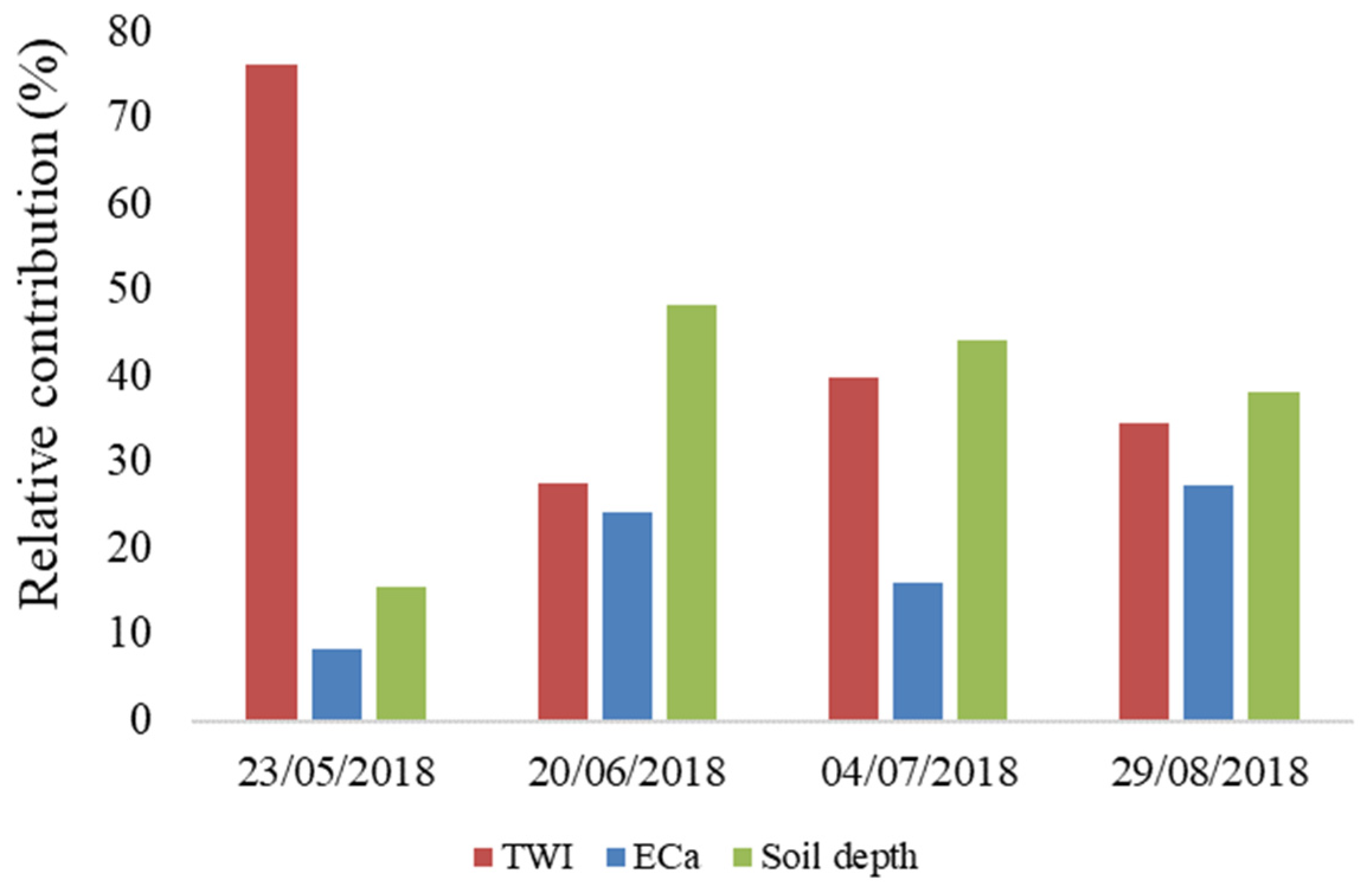
51]. Since our main objective in this study was to delineate MZs for precision irrigation purposes, we calculated the relative influence of three soil and topographic variables on the water status in the vineyard using extended measurements of Ψstem at four phenological stages (Figure 4). Results showed a clear, strong influence of TWI on Ψstem measurements at the beginning of the season while, as the season progressed, soil depth and ECa had higher or similar influence. Since none of the soil or topographic variables showed a constant relative influence on vine water status, MZ delineation in this vineyard appears to be not static. The dynamics of MZs with constant, pre-defined boundaries were tested to promote understanding of irrigation requirements under varied constraints and objectives regarding canopy size, water deficit stress and fruit quality.
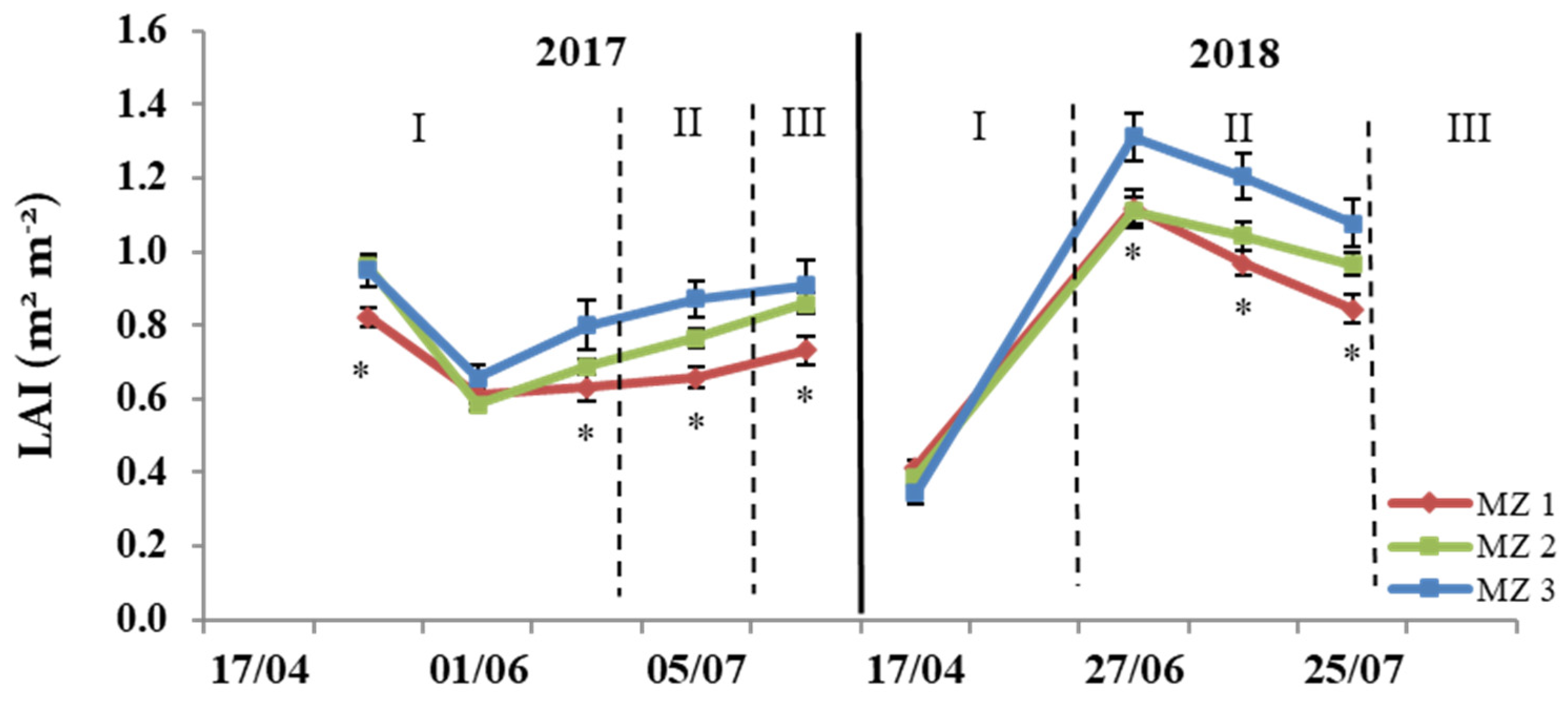
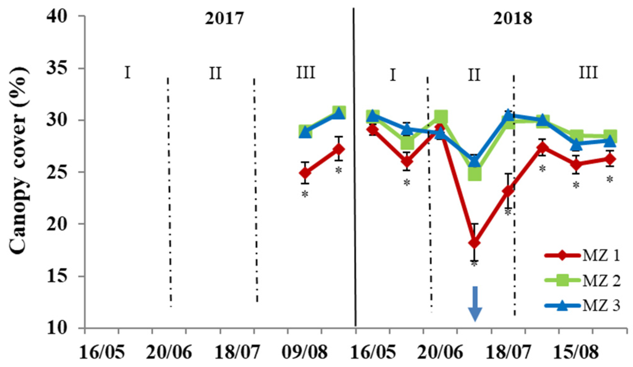
Vine vigor measurements revealed season-to-season differences with relatively higher LAI values during 2018 due to the greater spring precipitation (70.4 mm compared to 17.2 mm in 2017 between 1 March and 15 May each year), and differences between field measurements and remote sensing variables. Canopy cover results (Figure 8; Table A3) revealed differences between MZ1 and MZ2 and three in most cases while LAI results indicated that MZ3 values were highest, with smaller differences between MZs. The relations between LAI and canopy cover in the vineyard have rarely been studied. Though a few examples of ground-measured LAI–NDVI relationships have been published [52], none of them showed a strong correlation between the variables. It is assumed that LAI is more sensitive to vine vigor and can serve well as a parameter for irrigation scheduling in vineyards [53,54]. Moreover, LAI has been shown to be a particularly dominant factor influencing vine evapotranspiration [55].
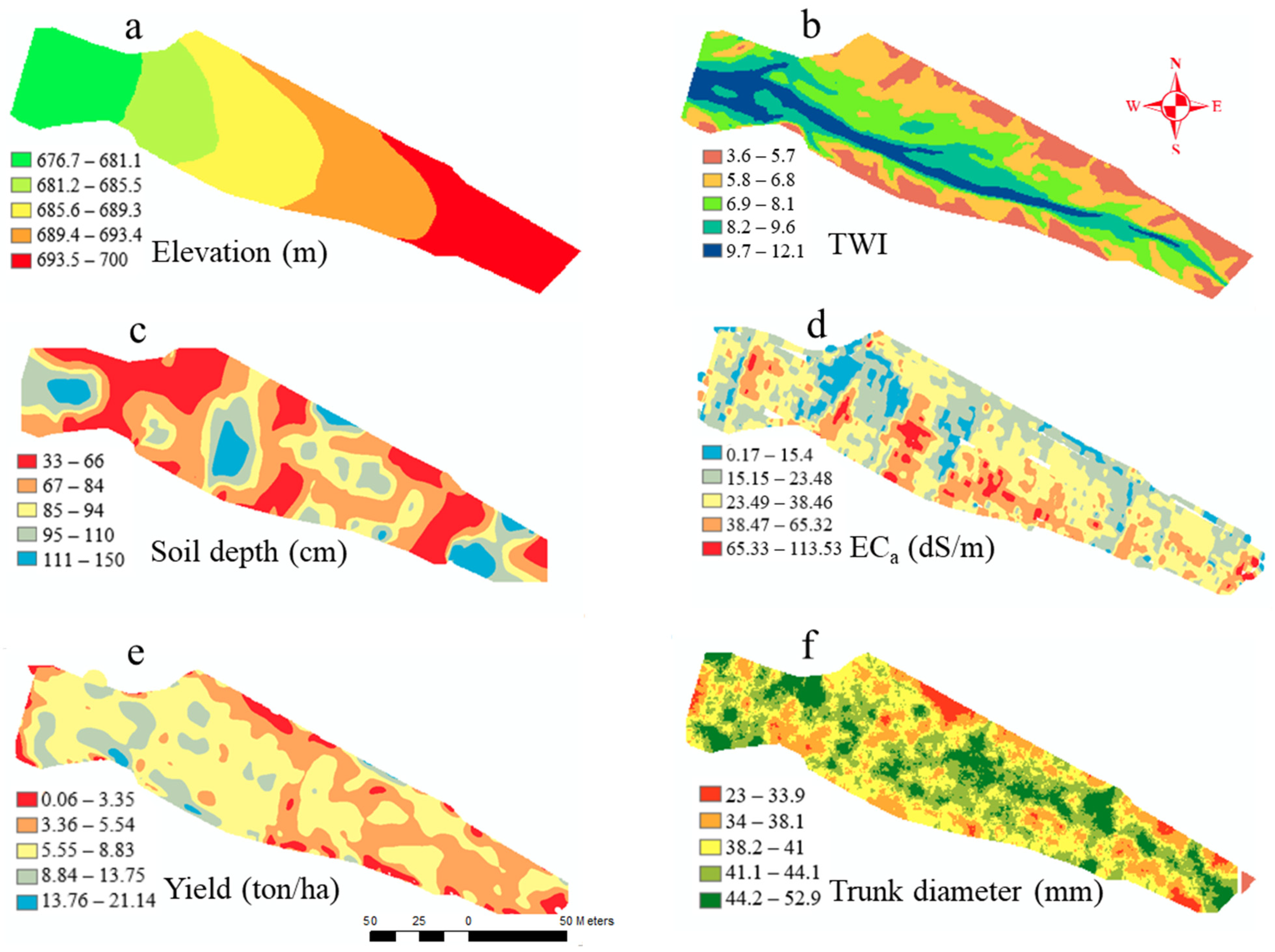
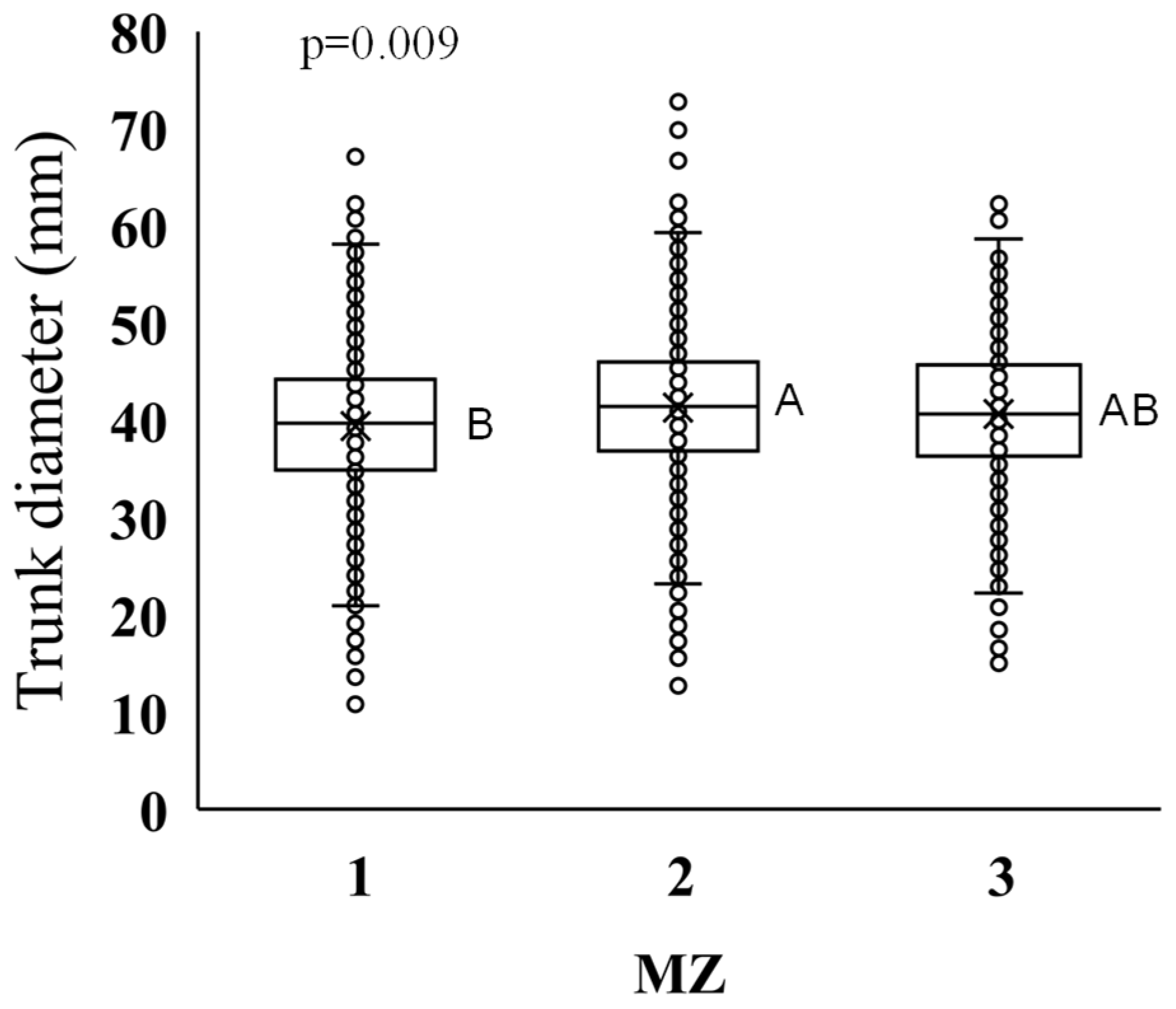
Trunk diameter represents the cumulated effect of vineyard variability on vine vigor. Figure 7 shows an intermediate effect of TWI on MZ3 average trunk diameter. It is well established that the most pronounced and rapid trunk growth occurs from flowering until veraison, followed by a decrease in trunk diameter as fruit starts ripening. Intrigliolo and Castel [56] suggested that the increase in trunk diameter is related to a strong connection between water availability from flowering to veraison, and the decrease in trunk diameter is related to carbohydrate demands of fruit and canopy from veraison onwards. This theory can explain the accumulated, multiyear effect in MZ3, which experienced high soil water availability leading to a high trunk diameter and a larger canopy at the beginning of the season, followed by a decrease in trunk diameter at the end of season.
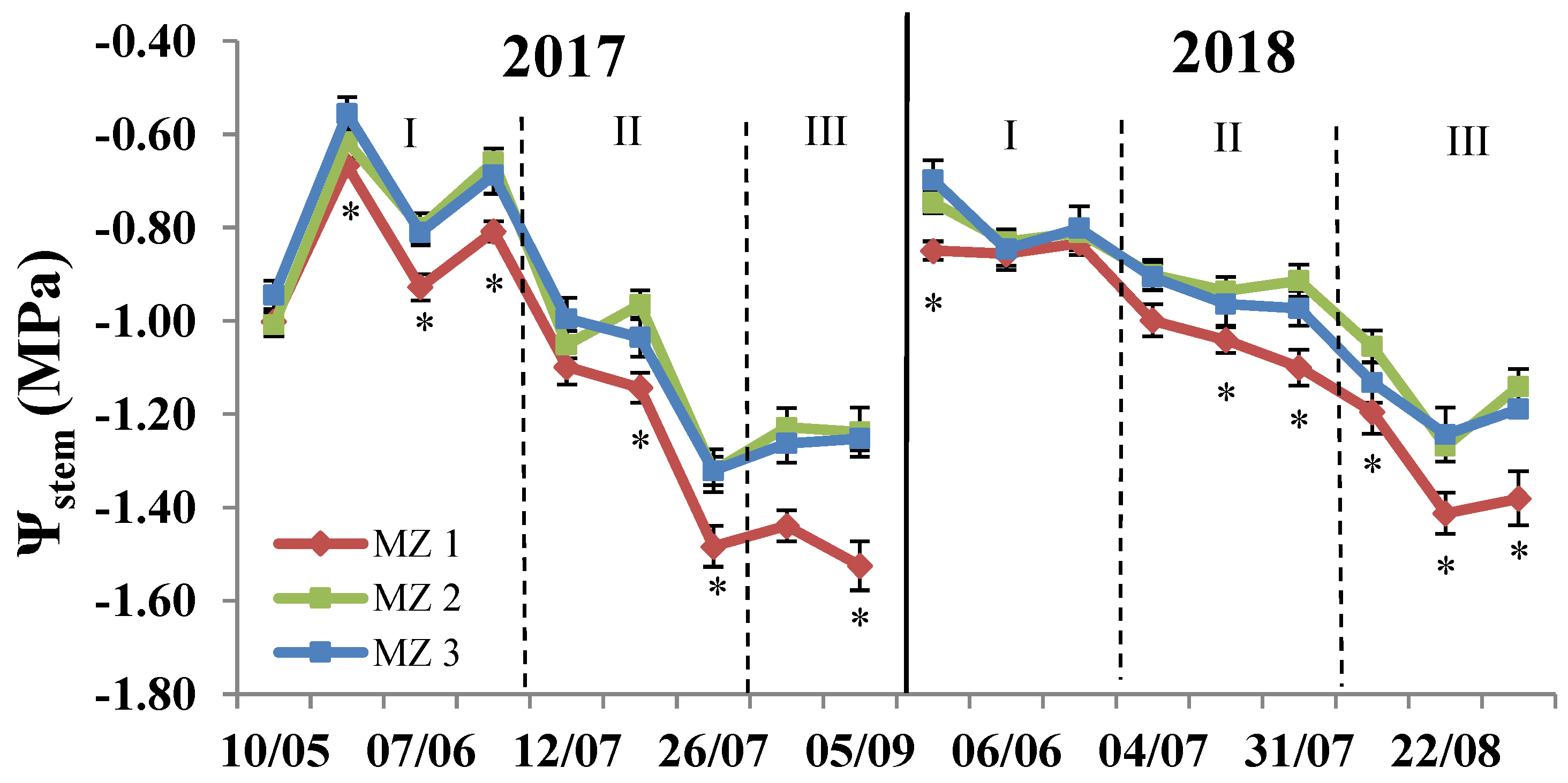
Vine vigor as revealed from LAI values indicated for high water availability in MZ3, which correspond with the TWI division and its high wetness index. Accordingly, it could be further expected that Ψstem values would be less negative than MZ2. Yet, in overall, Ψstem values in MZ3 were very similar to MZ2. The Ψstem trend of MZ3 at the beginning of each season indicates minimal water deficit stress, i.e., higher Ψstem, while at the end of the season the water status of MZ3 was similar to or slightly less than that of MZ2 (Figure 9; 
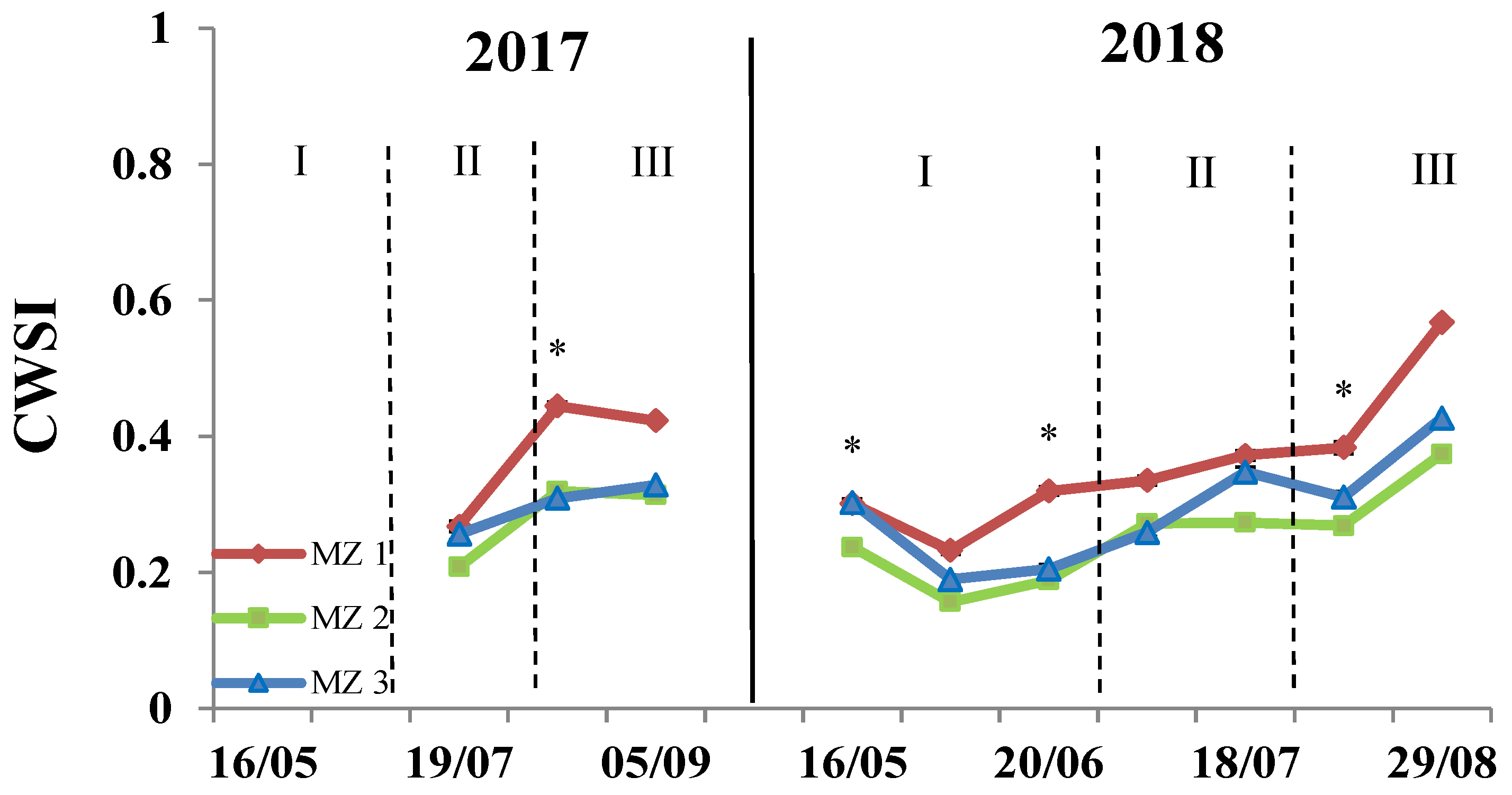
Table 2). Relation between proximal field and remotely sensed water stress measurements was more persistent than that of the vine vigor variables. The trend of CWSI in MZ3 revealed even larger differences. At the beginning of the season, MZ3 was at the lowest water deficit, i.e., lower CWSI, but at the end of the season its water status indicated intermediate water deficit stress (Figure 11). These findings lead to two important conclusions. First, that water status in MZ3 is a result of a complex interaction between water availability and vine vigor development and thus follows a dynamic temporal pattern. Such a dynamic trend may exist in other zones within vineyards as a function of high wetness index. Second, that remote sensing offers strong and important tools for water status measurements for precision irrigation purposes.
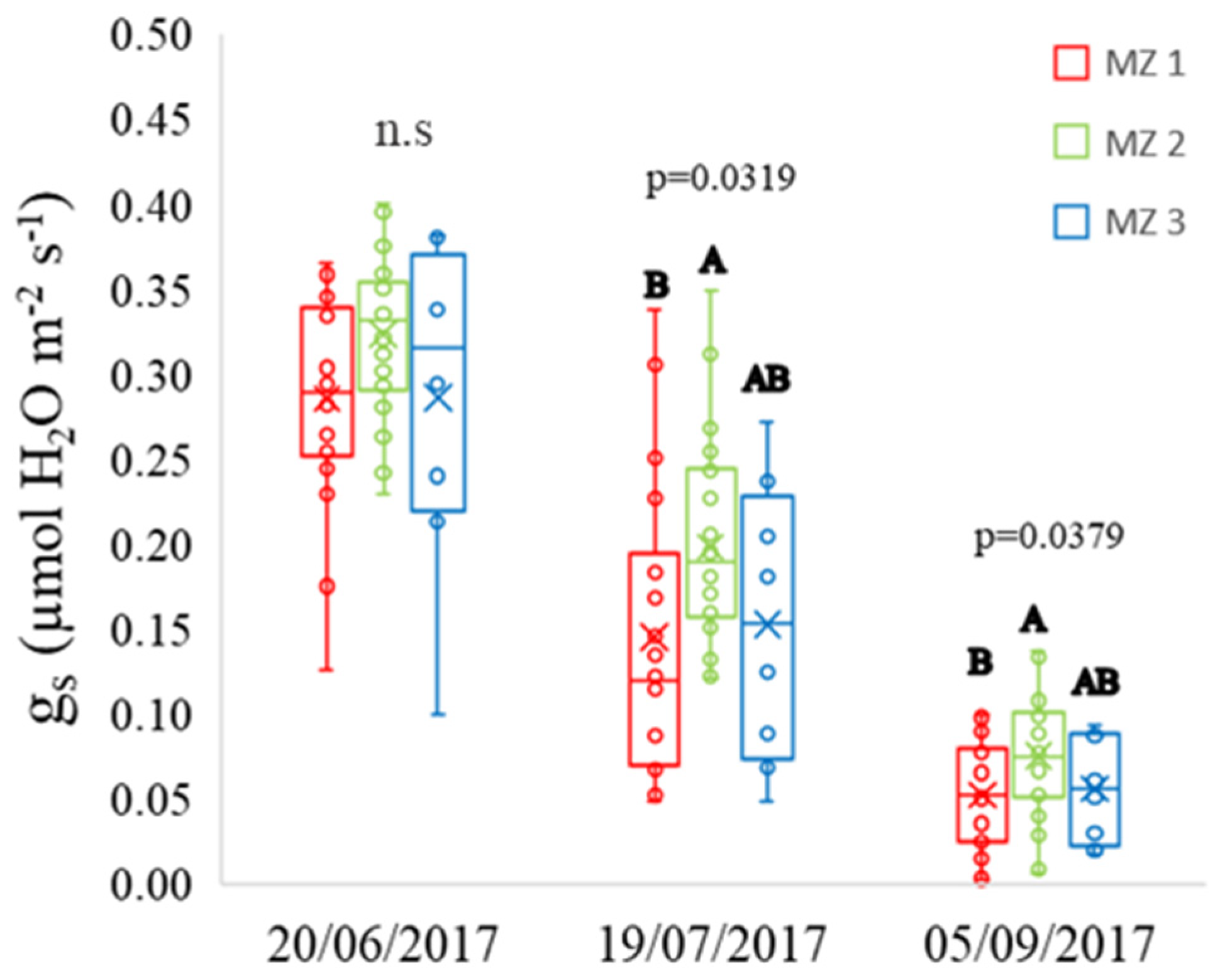
Previous studies have suggested that high soil and plant water availability can lead to larger canopies and consequently to greater water consumption and water stress at the end of the season [17,55]. Stomatal conductance results showed differences between MZ1 and MZ2 at stages II and III while MZ3 did not differ from any of the other MZs (Figure 10). These results are in agreement with remote sensing water status variable CWSI, showing the same intermediate status of MZ3 at stages II and III (Figure 11).
The spatial variability in TWI reflected the variability of grapevine physiology at the beginning of the season (stage I and partially stage II) but not at the end of season. Water deficit stress was not consistently different along the season between MZs in contrast to the results of Yu et al. [57] who delineated a ‘Cabernet Sauvignon’ vineyard in Ca, USA into 2 MZs based on Ψstem integrals. Differences between vineyards can be explained by heterogenic soil texture, soil depth and seasonal evaporative demand. As above-mentioned, while dynamic MZs have been studied in field crops [42,50,51], there is little known regarding orchards or vineyards. The approach requires continuous usage of reliable tools to assess spatiotemporal variation of plant vigor and vine water status. While remote sensing tools to evaluate vine water status and stress have been the subject of many studies [24,58,59,60], remote tools to sense vine vigor have been left behind. Assessment of canopy size using satellite imagery [61] has been attempted using a 3D canopy surface model [62] or image processing algorithms [63].
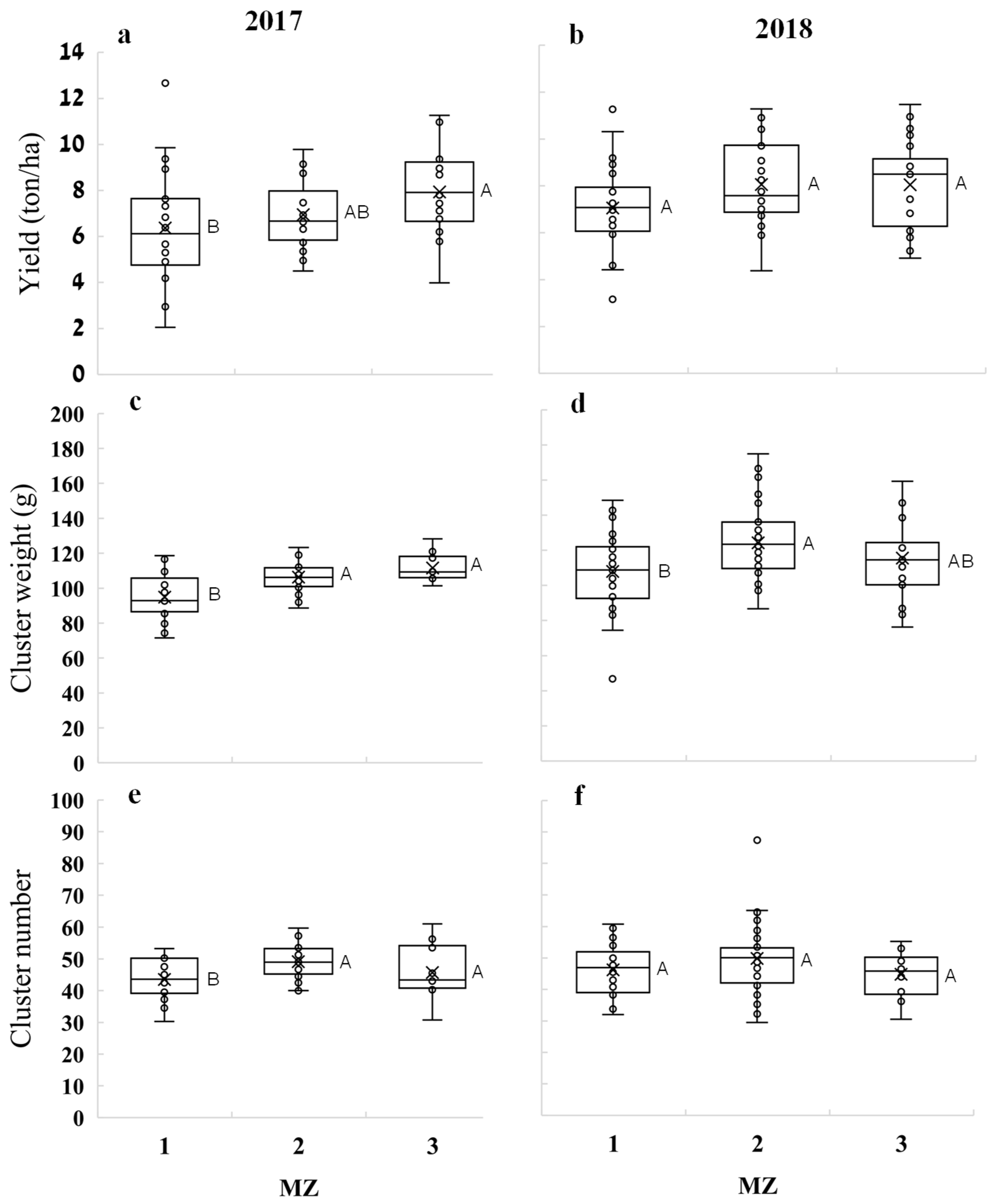
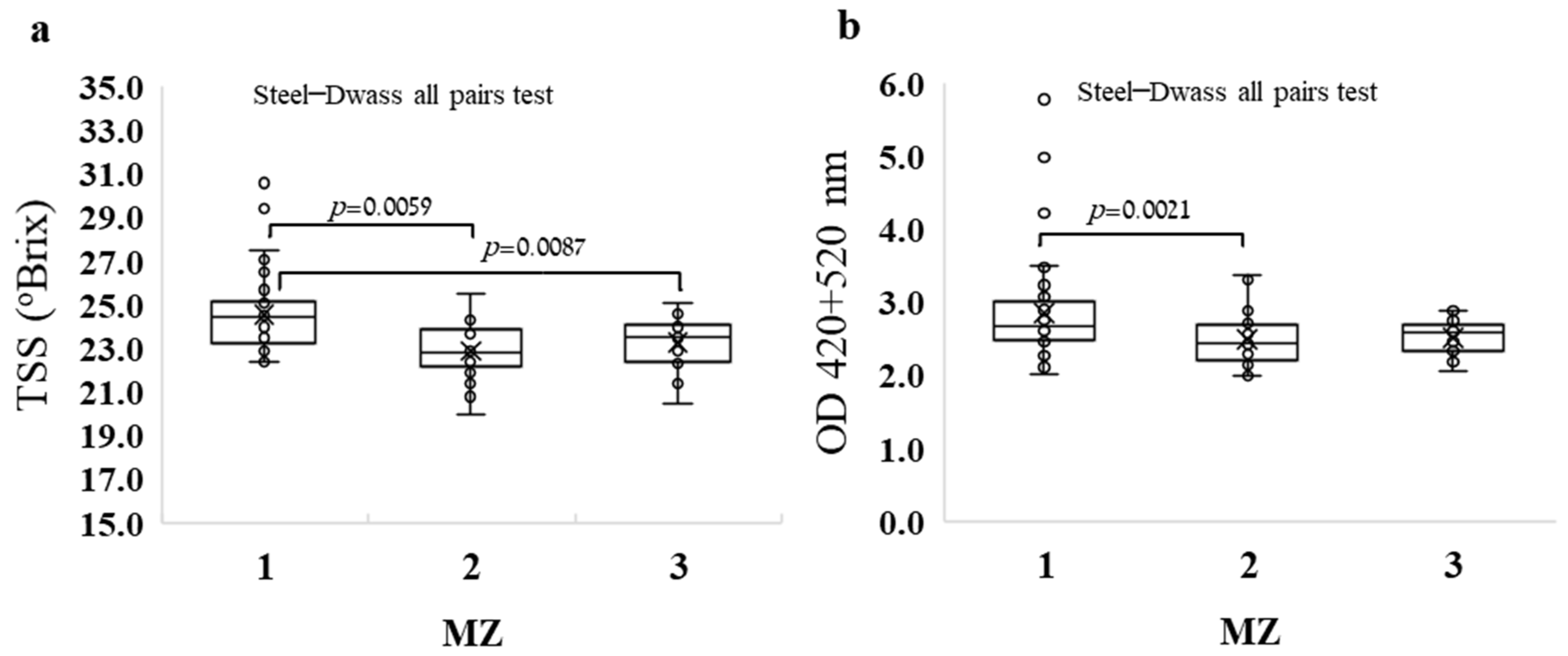
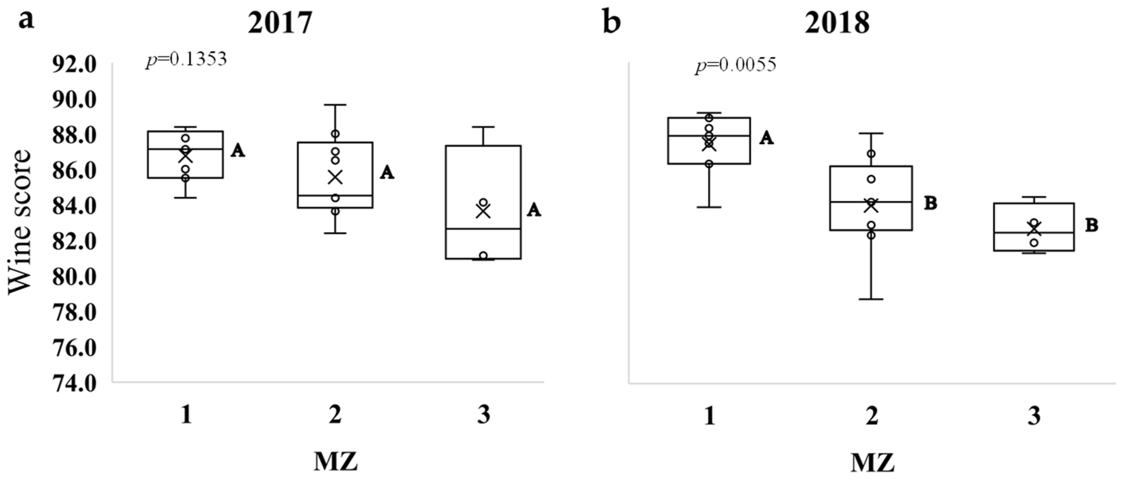
Results of yield and fruit quality show that vines under similar irrigation can respond uniquely as a function of location and spatial conditions. MZ1, the most distant from the wadi and steepest slope, was characterized by lower trunk diameter, LAI, and canopy cover on most of the measurement days (p < 0.05). MZ1 also demonstrated the greatest water deficit stress, eventually resulting in the lowest yield, highest TSS, fruit skin color and the highest wine score (n.s in 2017). Although we measured some differences in vine vigor between MZ3 and MZ2 during the 2017–2018 seasons, there were no significant differences between them in terms of fruit quantity, fruit quality and wine score.
Inducing water deficit stress in vineyards during stage III is favorable for quality red wine production, and has become a common practice in vineyards [21]. In an irrigation study in Israel, it was proved that providing regulated deficit irrigation (RDI) combining higher irrigation at stage I and lower irrigation at stage III has the potential to generate an optimal balance between vegetative growth, yield and wine with enhanced color and aroma compounds [16,17]. In this sense, zones within a vineyard with higher plant available water should be treated with unique RDI strategies. On one hand, this could improve water use in the vineyard, on the other, it could drive site-specific agrotechnical practices, particularly regarding canopy management.
Certainly, the future of precision irrigation will include utilization of accurate and feasible remote sensing tools. Additional studies should therefore consider MZ dynamics within vineyards, based on within season, continuous remote sensing retrievals.

5. Conclusions

We provided evidence for the relations between geomorphological spatial attributes of a vineyard and vine physiological response from early season vine vigor to wine quality. We showed the existence of temporal-dynamic MZs in our study vineyard. Understanding the relationships between soil water availability, vine vigor and water stress can improve irrigation decisions. TWI was successful in determining MZs in the current study and could serve as a cost effective, key factor for MZ delineation in other typical vineyards in semiarid regions where topography is spatially varied and winter and spring precipitation are important to vine growth and development and to irrigation management.

Author Contributions

Conceptualization, I.B., Y.C. and Y.N.; methodology, I.B., Y.C., Y.N., V.A., N.O.-L.; software, E.G.; validation, I.B., J.M.G. and A.P.; formal analysis, I.B.; investigation, I.B.; resources, V.A., Y.C., A.B.-G. and Y.N.; data curation, E.G. and A.P.; writing—original draft preparation, I.B.; writing—review and editing, I.B., Y.C., A.B.-G., Y.N., J.M.G., N.O.-L., A.P., E.G.; visualization, I.B.; supervision, Y.C., Y.N. and J.M.G. All authors have read and agreed to the published version of the manuscript.

Funding

This research is a part of the “Eugene Kendel” Project for Development of Precision Drip Irrigation funded via the Ministry of Agriculture and Rural Development in Israel (Grant No. 20-12-0030). The project has also received funding from the European Union’s Horizon 2020 research and innovation program under Project SHui, grant agreement No 773903.

Acknowledgments

We wish to thank Carmel winery for the vineyard contribution, and the agriculture division of ‘Carmel Winery’: Dror Dotan, Sarel Munitz, Avi Yehuda and David Twito. The authors wish to specially thank Ben Hazut, Matan Golomb and Doron Kleiman for their helpful assistance and accurate field measurements. The authors thank also to Oholi’av Keisar and Guy Lidor (ARO), for conducting the imaging campaigns.

Conflicts of Interest

The authors declare no conflict of interest.

Appendix A

Table A1. Leaf area index in each management zone (MZ) during 2017 and 2018. Each value is the mean of 22, 28 and 10 replicates for MZ 1, 2 and 3, respectively. The value of each replicate was the average of the measurements of two adjacent sample vines. Data were analyzed using ANOVA. Different letters represent significant differences among MZs, means were separated using the Tukey–Kramer HSD test (α = 0.05).
MZ17/0501/0614/0605/0716/08
201710.82 B0.61 A0.63 B0.66 B0.73 B
20.96 A0.59 A0.69 AB0.77 A0.86 A
30.95 A0.66 A0.80 A0.87 A0.91 A
17/0427/0611/0725/07
201810.41 A1.12 AB0.97 B0.85 B
20.39 A1.11 B1.04 AB0.97 AB
30.35 A1.31 A1.21 A1.08 A
Table A2. Midday stem water potential in each management zone (MZ) during 2017 and 2018. Each value is the mean of 22, 28 and 10 replicates for MZ 1, 2 and 3, respectively. The value of each replicate was the average of the measurements of two adjacent sample vines. Data were analyzed by ANOVA. Different letters represent significant differences among MZs, means were separated using the Tukey–Kramer HSD test (α = 0.05).
MZ10/0524/0507/0628/0612/0719/0726/0709/0805/09
20171−1.00 A−0.67 B−0.93 B−0.81 B−1.10 A−1.14 B−1.48 B−1.37 A−1.53 B
2−1.01 A−0.62 AB−0.80 A−0.66 A−1.05 A−0.96 A−1.32 A−1.23 A−1.24 A
3−0.94 A−0.56 A−0.81 AB−0.69 AB−1.00 A−1.04 AB−1.32 AB−1.26 A−1.25 A
23/0506/0620/0604/0718/0731/0715/0822/0829/08
20181−0.85 B−0.86 A−0.83 A−1.00 A−1.04 B−1.10 B−1.20 B−1.41 B−1.38 B
2−0.75 A−0.83 A−0.81 A−0.90 A−0.94 A−0.91 A−1.05 A−1.27 A−1.14 A
3−0.70 A−0.85 A−0.80 A−0.91 A−0.96 AB−0.97 AB−1.13 AB−1.24 AB−1.19 AB
Table A3. Canopy cover for each management zone (MZ) during 2017 and 2018. Measurement was done first by calculating NDVI in vine rows, then calculating the canopy coverage of each MZ. Each value is the mean of 22 random points created to account for spatial autocorrelation. Data were analyzed by ANOVA. Different letters represent significant differences among MZs, means were separated using the Tukey–Kramer HSD test (α = 0.05).
MZ09/0805/09
2017124.9 B27.2 B
229.0 A30.8 A
328.9 A30.7 A
16/0506/0620/0604/0718/0731/0715/0829/0826/09
2018129.09 A26.03 B29.32 A18.24 B23.20 B27.38 B25.74 B26.31 B24.11 B
230.41 A27.88 AB30.38 A24.82 A29.85 A29.91 A28.52 A28.46 A26.72 A
330.46 A29.20 A28.80 A26.11 A30.53 A30.06 A27.72 AB28.02 AB25.93 AB

References

  1. Brillante, L.; Bois, B.; Lévêque, J.; Mathieu, O. Variations in Soil-Water Use by Grapevine According to Plant Water Status and Soil Physical-Chemical Characteristics-A 3D Spatio-Temporal Analysis. Eur. J. Agron. 2016, 77, 122–135. [Google Scholar] [CrossRef]
  2. Ortuani, B.; Facchi, A.; Mayer, A.; Bianchi, D.; Brancadoro, L. Assessing the Effectiveness of Variable-Rate Drip Irrigation on Water Use Efficiency in a Vineyard in Northern Italy. Water 2019, 11, 1964. [Google Scholar] [CrossRef] [Green Version]
  3. Doerge, T.A. Management Zone Concepts. Site Specif. Manag. Guidel. 1999, 4. Available online: https://www.ipni.net/publication/ssmg.nsf/0/C0D052F04A53E0BF852579E500761AE3/$FILE/SSMG-02.pdf (accessed on 2 April 2021).
  4. Van Leeuwen, C.; Goutouly, J.; Azaïs, C.; Marguerit, E.; Roby, J.; Chone, X.; Germain, C. Intra-Block Variations of Vine Water Status in Time and Space. Available online: https://www.researchgate.net/profile/Cornelis-Van-Leeuwen/publication/278804292_Intraplot_variations_of_vine_water_status_in_time_and_space/links/57daadac08ae72d72ea35924/Intra-plot-variations-of-vine-water-status-in-time-and-space.pdf (accessed on 17 April 2021).
  5. Bramley, R.G.V.; Trought, M.C.T.; Praat, J.P. Vineyard Variability in Marlborough, New Zealand: Characterising Spatial and Temporal Changes in Fruit Composition and Juice Quality in the Vineyard. Aust. J. Grape Wine Res. 2011, 17, 72–78. [Google Scholar] [CrossRef]
  6. Ortega-Blu, R.; Molina-Roco, M. Evaluation of Vegetation Indices and Apparent Soil Electrical Conductivity for Site-Specific Vineyard Management in Chile. Precis. Agric. 2016, 17, 434–450. [Google Scholar] [CrossRef]
  7. Arnó, J.; Bordes, X.; Ribes-Dasi, M.; Blanco, R.; Rosell, J.R.; Esteve, J. Obtaining Grape Yield Maps and Analysis of Within-Field Variability in Raimat (Spain). Precis. Agric. 2005, 5, 899–906. [Google Scholar]
  8. Santesteban, L.G.; Guillaume, S.; Royo, J.B.; Tisseyre, B. Are Precision Agriculture Tools and Methods Relevant at the Whole-Vineyard Scale? Precis. Agric. 2011, 14, 302–311. [Google Scholar] [CrossRef] [Green Version]
  9. Ohana-Levi, N.; Bahat, I.; Peeters, A.; Shtein, A.; Netzer, Y.; Cohen, Y.; Ben-Gal, A. A Weighted Multivariate Spatial Clustering Model to Determine Irrigation Management Zones. Comput. Electron. Agric. 2019, 162, 719–731. [Google Scholar] [CrossRef]
  10. Matese, A.; Baraldi, R.; Berton, A.; Cesaraccio, C.; Di Gennaro, S.F.; Duce, P.; Facini, O.; Mameli, M.G.; Piga, A.; Zaldei, A. Estimation of Water Stress in Grapevines Using Proximal and Remote Sensing Methods. Remote Sens. 2018, 10, 114. [Google Scholar] [CrossRef] [Green Version]
  11. Jasse, A.; Poblete-echeverría, C.; Berry, A.; Aleixandre-tudo, J.L.; Poblete-echeverría, C. Intra-Block Spatial and Temporal Variability of Plant Water Status and Its Effect on Grape and Wine Parameters. Agric. Water Manag. 2020, 246, 106696. [Google Scholar] [CrossRef]
  12. Sørensen, R.; Zinko, U.; Seibert, J. On the Calculation of the Topographic Wetness Index: Evaluation of Different Methods Based on Field Observations. Hydrol. Earth Syst. Sci. 2006, 10, 101–112. [Google Scholar] [CrossRef] [Green Version]
  13. Bui, D.T.; Khosravi, K.; Shahabi, H.; Daggupati, P.; Adamowski, J.F.; Melesse, A.M.; Pham, B.T.; Pourghasemi, H.R.; Mahmoudi, M.; Bahrami, S.; et al. Flood Spatial Modeling in Northern Iran Using Remote Sensing and GIS: A Comparison between Evidential Belief Functions and Its Ensemble with a Multivariate Logistic Regression Model. Remote Sens. 2019, 11, 1589. [Google Scholar] [CrossRef] [Green Version]
  14. Ohana-Levi, N.; Knipper, K.; Kustas, W.P.; Anderson, M.C.; Netzer, Y.; Gao, F.; Alsina, M.d.M.; Sanchez, L.A.; Karnieli, A. Using Satellite Thermal-Based Evapotranspiration Time Series for Defining Management Zones and Spatial Association to Local Attributes in a Vineyard. Remote Sens. 2020, 12, 2436. [Google Scholar] [CrossRef]
  15. Choné, X.; van Leeuwen, C.; Dubourdieu, D.; Guadilleare, J.P. Stem Water Potential Is a Sensitive Indicator of Grapevine Water Status. Ann. Bot. 2001, 87, 477–483. [Google Scholar] [CrossRef] [Green Version]
  16. Munitz, S.; Netzer, Y.; Schwartz, A. Sustained and Regulated Deficit Irrigation of Field-Grown Merlot Grapevines. Aust. J. Grape Wine Res. 2017, 23, 87–94. [Google Scholar] [CrossRef]
  17. Netzer, Y.; Munitz, S.; Shtein, I.; Schwartz, A. Structural Memory in Grapevines: Early Season Water Availability Affects Late Season Drought Stress Severity. Eur. J. Agron. 2019, 105, 96–103. [Google Scholar] [CrossRef]
  18. Acevedo-Opazo, C.; Ortega-farias, S.; Fuentes, S. Effects of Grapevine (Vitis Vinifera L.) Water Status on Water Consumption, Vegetative Growth and Grape Quality: An Irrigation Scheduling Application to Achieve Regulated Deficit Irrigation. Agric. Water Manag. 2010, 97, 956–964. [Google Scholar] [CrossRef]
  19. Van Leeuwen, C.; Tregoat, O.; Choné, X.; Bois, B.; Pernet, D.; Gaudillere, J.P. Vine Water Status Is a Key Factor in Grape Ripening and Vintage Quality for Red Bordeaux Wine. How Can It Be Assessed for Vineyard Management Purposes? Oeno One 2009, 43, 121–134. [Google Scholar] [CrossRef]
  20. Winkler, A.J.; Cook, J.A.; Kliewer, W.M.; Lider, L.A. Development and composition of grapes. In General Viticulture, 2nd ed.; University of California Press: Berkeley, CA, USA, 1974. [Google Scholar]
  21. Castellarin, S.D.; Matthews, M.A.; Di Gaspero, G.; Gambetta, G.A. Water Deficits Accelerate Ripening and Induce Changes in Gene Expression Regulating Flavonoid Biosynthesis in Grape Berries. Planta 2007, 227, 101–112. [Google Scholar] [CrossRef]
  22. Bellvert, J.; Zarco-Tejada, P.J.; Marsal, J.; Girona, J.; González-Dugo, V.; Fereres, E. Vineyard Irrigation Scheduling Based on Airborne Thermal Imagery and Water Potential Thresholds. Aust. J. Grape Wine Res. 2016, 22, 307–315. [Google Scholar] [CrossRef] [Green Version]
  23. Espinoza, C.Z.; Khot, L.R.; Sankaran, S.; Jacoby, P.W. High Resolution Multispectral and Thermal Remote Sensing-Based Water Stress Assessment in Subsurface Irrigated Grapevines. Remote Sens. 2017, 9, 961. [Google Scholar] [CrossRef] [Green Version]
  24. Sepúlveda-Reyes, D.; Ingram, B.; Bardeen, M.; Zúñiga, M.; Ortega-Farías, S.; Poblete-Echeverría, C. Selecting Canopy Zones and Thresholding Approaches to Assess Grapevine Water Status by Using Aerial and Ground-Based Thermal Imaging. Remote Sens. 2016, 8, 822. [Google Scholar] [CrossRef] [Green Version]
  25. Möller, M.; Alchanatis, V.; Cohen, Y.; Meron, M.; Tsipris, J.; Naor, A.; Ostrovsky, V.; Sprintsin, M.; Cohen, S. Use of Thermal and Visible Imagery for Estimating Crop Water Status of Irrigated Grapevine. J. Exp. Bot. 2007, 58, 827–838. [Google Scholar] [CrossRef] [PubMed] [Green Version]
  26. Santesteban, L.G.; Di Gennaro, S.F.; Herrero-Langreo, A.; Miranda, C.; Royo, J.B.; Matese, A. High-Resolution UAV-Based Thermal Imaging to Estimate the Instantaneous and Seasonal Variability of Plant Water Status within a Vineyard. Agric. Water Manag. 2017, 183, 49–59. [Google Scholar] [CrossRef]
  27. Rodríguez-Pérez, J.R.; Plant, R.E.; Lambert, J.J.; Smart, D.R. Using Apparent Soil Electrical Conductivity (ECa) to Characterize Vineyard Soils of High Clay Content. Precis. Agric. 2011, 12, 775–794. [Google Scholar] [CrossRef] [Green Version]
  28. Priori, S.; Martini, E.; Andrenelli, M.C.; Magini, S.; Agnelli, A.E.; Bucelli, P.; Biagi, M.; Pellegrini, S.; Costantini, E.A.C. Improving Wine Quality through Harvest Zoning and Combined Use of Remote and Soil Proximal Sensing. Soil Sci. Soc. Am. J. 2013, 77, 1338–1348. [Google Scholar] [CrossRef]
  29. Munitz, S.; Netzer, Y.; Shtein, I.; Schwartz, A. Water Availability Dynamics Have Long-Term Effects on Mature Stem Structure in Vitis Vinifera. Am. J. Bot. 2018, 105, 1443–1452. [Google Scholar] [CrossRef] [PubMed] [Green Version]
  30. Allen, R.G.; Pruitt, W.O.; Wright, J.L.; Howell, T.A.; Ventura, F.; Snyder, R.; Itenfisu, D.; Steduto, P.; Berengena, J.; Yrisarry, J.B.; et al. A Recommendation on Standardized Surface Resistance for Hourly Calculation of Reference ETo by the FAO56 Penman-Monteith Method. Agric. Water Manag. 2006, 81, 1–22. [Google Scholar] [CrossRef]
  31. Bahat, I.; Netzer, Y.; Ben-Gal, A.; Grünzweig, J.M.; Peeters, A.; Cohen, Y. Comparison of Water Potential and Yield Parameters under Uniform and Variable Rate Drip Irrigation in a Cabernet Sauvignon Vineyard. In Proceedings of the Precision Agriculture 2019-Papers Presented at the 12th European Conference on Precision Agriculture, ECPA 2019, Montpellier, France, 8–11 July 2019. [Google Scholar]
  32. Agricultural Research Organization (ARO). Volcani Institute, Israel, Developing Precision Irrigation Systems. Available online: https://volcani.maps.arcgis.com/home/index.html (accessed on 14 April 2021).
  33. Beven, K.J.; Kirkby, M.J. A Physically Based, Variable Contributing Area Model of Basin Hydrology. Hydrol. Sci. Bull. 1979, 24, 43–69. [Google Scholar] [CrossRef] [Green Version]
  34. Metcalfe, P.; Beven, K.; Freer, J. Package “Dynatopmodel”: Implementation of the Dynamic TOPMODEL Hydrological Model. R Packag. Version 1.2.1. 2018. Available online: https//CRAN.R-project.org/package=dynatopmodel (accessed on 30 May 2020).
  35. Corwin, D.L.; Lesch, S.M. Characterizing Soil Spatial Variability with Apparent Soil Electrical Conductivity: I. Survey Protocols. Comput. Electron. Agric. 2005, 46, 103–133. [Google Scholar] [CrossRef]
  36. Smart, D.R.; Schwass, E.; Lakso, A.; Morano, L. Grapevine Rooting Patterns: A Comprehensive Analysis and a Review. Am. J. Enol. Vitic. 2006, 57, 89–104. [Google Scholar]
  37. Netzer, Y.; Yao, C.; Shenker, M.; Bravdo, B.A.; Schwartz, A. Water Use and the Development of Seasonal Crop Coefficients for Superior Seedless Grapevines Trained to an Open-Gable Trellis System. Irrig. Sci. 2009, 27, 109–120. [Google Scholar] [CrossRef]
  38. Boyer, J.S. Measuring the Water Status of Plants and Soils; Academic Press: San Diego, CA, USA, 1995. [Google Scholar]
  39. Jackson, R.D.; Idso, S.B.; Reginato, R.J.; Pinter, P.J. Canopy Temperature as a Crop Water Stress Indicator. Water Resour. Res. 1981, 17, 1133–1138. [Google Scholar] [CrossRef]
  40. Meron, M.; Tsipris, J.; Orlov, V.; Alchanatis, V.; Cohen, Y. Crop Water Stress Mapping for Site-Specific Irrigation by Thermal Imagery and Artificial Reference Surfaces. Precis. Agric. 2010, 11, 148–162. [Google Scholar] [CrossRef]
  41. Rud, R.; Cohen, Y.; Alchanatis, V.; Levi, A.; Brikman, R.; Shenderey, C.; Heuer, B.; Markovitch, T.; Dar, Z.; Rosen, C.; et al. Crop Water Stress Index Derived from Multi-Year Ground and Aerial Thermal Images as an Indicator of Potato Water Status. Precis. Agric. 2014, 15, 273–289. [Google Scholar] [CrossRef]
  42. Cohen, Y.; Alchanatis, V.; Saranga, Y.; Rosenberg, O.; Sela, E.; Bosak, A. Mapping Water Status Based on Aerial Thermal Imagery: Comparison of Methodologies for Upscaling from a Single Leaf to Commercial Fields. Precis. Agric. 2017, 18, 801–822. [Google Scholar] [CrossRef]
  43. Hijmans, R.J.; Etten, J.; van Sumner, M.; Cheng, J.; Bevan, A.; Bevan, R.; Busetto, L.; Canty, M.; Forrest, D.; Ghosh, A.; et al. Package “Raster”. Available online: https://rspatial.org/raster/ (accessed on 31 October 2020).
  44. Compendium of International Methods of Analysis of Wines and Musts. Organisation International de la Vigne (OIV). Available online: https://www.oiv.int/en/technical-standards-and-documents/methods-of-analysis/compendium-of-international-methods-of-analysis-of-wines-and-musts-2-vol (accessed on 11 August 2020).
  45. Hastie, T.; Tibshirani, R.; Friedman, J. Boosting and Additive Trees. In The Elements of Statistical Learning-Data Mining, Inference, and Prediction; Springer: Berlin, Germany, 2009; Volume 2, Available online: https://books.google.co.il/books/about/The_Elements_of_Statistical_Learning.html?id=VRzITwgNV2UC&redir_esc=y (accessed on 2 February 2021).
  46. Lowrance, C.; Fountas, S.; Liakos, V.; Vellidis, G. EZZone—An Online Tool for Delineating Management Zones. In Proceedings of the 13th International Conference on Precision Agriculture, St. Louis, MO, USA, 31 July–3 August 2016; pp. 1–17. [Google Scholar]
  47. R Core Team. R: A Language and Environment for Statistical Computing. Available online: https://www.R-project.org/ (accessed on 1 September 2020).
  48. Cohen, Y.; Alchanatis, V.; Prigojin, A.; Levi, A.; Soroker, V.; Cohen, Y. Use of Aerial Thermal Imaging to Estimate Water Status of Palm Trees. Precis. Agric. 2012, 13, 123–140. [Google Scholar] [CrossRef]
  49. Israel Meteorological Service Multiannual Climate Data 1981–2000. Available online: https://ims.data.gov.il/ims/1 (accessed on 2 October 2020).
  50. O’Shaughnessy, S.A.; Evett, S.R.; Colaizzi, P.D. Dynamic Prescription Maps for Site-Specific Variable Rate Irrigation of Cotton. Agric. Water Manag. 2015, 159, 123–138. [Google Scholar] [CrossRef]
  51. Fontanet, M.; Scudiero, E.; Skaggs, T.H.; Fernàndez-garcia, D.; Ferrer, F.; Rodrigo, G.; Bellvert, J. Dynamic Management Zones for Irrigation Scheduling. Agric. Water Manag. 2020, 238, 106207. [Google Scholar] [CrossRef]
  52. Johnson, L.F. Temporal Stability of an NDVI-LAI Relationship in a Napa Valley Vineyard. Aust. J. Grape Wine Res. 2003, 9, 96–101. [Google Scholar] [CrossRef]
  53. Munitz, S.; Schwartz, A.; Netzer, Y. Water Consumption, Crop Coefficient and Leaf Area Relations of a Vitis Vinifera Cv. “Cabernet Sauvignon” Vineyard. Agric. Water Manag. 2019, 219, 86–94. [Google Scholar] [CrossRef]
  54. Picón-Toro, J.; González-Dugo, V.; Uriarte, D.; Mancha, L.A.; Testi, L. Effects of Canopy Size and Water Stress over the Crop Coefficient of a “Tempranillo” Vineyard in South-Western Spain. Irrig. Sci. 2012, 30, 419–432. [Google Scholar] [CrossRef] [Green Version]
  55. Ohana-Levi, N.; Munitz, S.; Ben-Gal, A.; Netzer, Y. Evaluation of Within-Season Grapevine Evapotranspiration Patterns and Drivers Using Generalized Additive Models. Agric. Water Manag. 2020, 228, 105808. [Google Scholar] [CrossRef]
  56. Intrigliolo, D.S.; Castel, J.R. Evaluation of Grapevine Water Status from Trunk Diameter Variations. Irrig. Sci. 2007, 26, 49–59. [Google Scholar] [CrossRef] [Green Version]
  57. Yu, R.; Brillante, L.; Martínez-Lüscher, J.; Kurtural, S.K. Spatial Variability of Soil and Plant Water Status and Their Cascading Effects on Grapevine Physiology Are Linked to Berry and Wine Chemistry. Front. Plant Sci. 2020, 11, 790. [Google Scholar] [CrossRef] [PubMed]
  58. Maes, W.; Steppe, K. Estimating Evapotranspiration and Drought Stress with Ground-Based Thermal Remote Sensing in Agriculture: A Review. J. Exp. Bot. 2012, 63, 4671–4712. [Google Scholar] [CrossRef] [PubMed] [Green Version]
  59. Bellvert, J.; Marsal, J.; Girona, J.; Zarco-Tejada, P.J. Seasonal Evolution of Crop Water Stress Index in Grapevine Varieties Determined with High-Resolution Remote Sensing Thermal Imagery. Irrig. Sci. 2014, 33, 81–93. [Google Scholar] [CrossRef]
  60. Pou, A.; Diago, M.P.; Medrano, H.; Baluja, J.; Tardaguila, J. Validation of Thermal Indices for Water Status Identification in Grapevine. Agric. Water Manag. 2014, 134, 60–72. [Google Scholar] [CrossRef]
  61. Johnson, L.F.; Roczen, D.E.; Youkhana, S.K.; Nemani, R.R.; Bosch, D.F. Mapping Vineyard Leaf Area with Multispectral Satellite Imagery. Comput. Electron. Agric. 2003, 38, 33–44. [Google Scholar] [CrossRef]
  62. Kalisperakis, I.; Stentoumis, C.; Grammatikopoulos, L.; Karantzalos, K. Leaf Area Index Estimation in Vineyards from UAV Hyperspectral Data, 2D Image Mosaics and 3D Canopy Surface Models. Int. Arch. Photogramm. Remote Sens. Spat. Inf. Sci. 2015, 40, 299–303. [Google Scholar] [CrossRef] [Green Version]
  63. Mora, M.; Avila, F.; Carrasco-Benavides, M.; Maldonado, G.; Olguín-Cáceres, J.; Fuentes, S. Automated Computation of Leaf Area Index from Fruit Trees Using Improved Image Processing Algorithms Applied to Canopy Cover Digital Photographies. Comput. Electron. Agric. 2016, 123, 195–202. [Google Scholar] [CrossRef] [Green Version]
Figure 1. The study site: (a) vineyard location within Israel; and (b) Mevo-Beitar experimental vineyard. Management cells are represented in black squares with different English alphabet letters (n = 20). Measurement vines are marked as blue dots (n = 120), and yield-monitored vines (n = 240) as blank open circles.
Remotesensing 13 01636 g001
Figure 2. Spatial maps of (a) elevation (masl), (b) topographic wetness index (TWI), (c) soil depth (cm), (d) apparent electrical conductivity (ECa) at 0–75 cm depth, (e) yield from 2017 (ton/ha) and (f) trunk diameter (mm).
Remotesensing 13 01636 g002
Figure 3. Maps of Ψstem (MPa) on 4 measurement days: (a) fruit set 23 May 2018; (b) bunch closure 20 June 2018; (c) veraison 4 July 2018 and (d) harvest 29 August 2018. Target Ψstem values for each date are shown in brackets.
Remotesensing 13 01636 g003
Figure 4. Relative contribution of soil and terrain variables to Ψstem at fruit set (23 May 2018), bunch closure (20 June 2018), veraison (4 July 2018) and harvest (29 August 2018). RMSE ranged between 0.06 at early season and 0.18 at the end of season. TWI is topographical wetness index and ECa is apparent electrical conductivity.
Remotesensing 13 01636 g004
Figure 5. Vineyard delineation into three management zones (MZs) based on topographical wetness index: MZ1 (red), MZ2 (green) and MZ3 (blue). Management cells are represented by black squares with different letters. Measurement vines are marked as blue dots.
Remotesensing 13 01636 g005
Figure 6. Seasonal course of leaf area index (LAI) of vines in the management zones (MZs) during 2017 and 2018. Each point is the mean of 44, 56 and 20 vines for MZ 1, 2 and 3, respectively ± SE. Asterisks represent significant differences among MZs using ANOVA (α = 0.05).
Remotesensing 13 01636 g006
Figure 7. Boxplots presenting the distribution of trunk diameter of vines in the three management zones (MZs), as measured in January 2017. Different letters indicate significant differences as analyzed by ANOVA (α = 0.05).
Remotesensing 13 01636 g007
Figure 8. Seasonal course of canopy cover of the vines in the management zones (MZs) during 2017 and 2018. Measurement was conducted first by calculating NDVI in vine rows, then calculating the canopy coverage of every MZ. Each point is the mean of 22 random points created to account for spatial autocorrelation. The blue arrow indicates date of canopy trimming. Asterisks represent significant differences among MZs using ANOVA (α = 0.05).
Remotesensing 13 01636 g008
Figure 9. Seasonal course of midday stem water potential (Ψstem) of vines in the management zones (MZs) during 2017 and 2018. Each point is the mean of 44, 56 and 20 vines for MZ 1, 2 and 3, respectively ± SE. Asterisks represent significant differences among MZs as determined by ANOVA (α = 0.05).
Remotesensing 13 01636 g009
Figure 10. Stomatal conductance to water vapor (gs) on three days, representing different phenological stages: 20 June 2017—bunch closure, 19 July 2017—veraison and 5 September 2017—harvest. Data were measured in the western block (MCs A–J) around solar noon. Steel–Dwass test was performed in 20 June 2017. In other cases, significant differences among MZs were evaluated by ANOVA (α = 0.05). Different letters represent significant differences among MZs, means were separated using the Tukey–Kramer HSD test (α = 0.05). n.s represents not significant.
Remotesensing 13 01636 g010
Figure 11. Seasonal course of crop water stress index (CWSI) of vines in the management zones during 2017 and 2018. Each point is the mean of 2031, 2126 and 1364 vine polygons for MZ 1, 2 and 3, respectively ± SE. The value of each replicate was the average of the lowest 33% of vine’s polygon. Asterisks represent significant differences among MZs using ANOVA (α = 0.05).
Remotesensing 13 01636 g011
Figure 12. Boxplot of yield and fruit quality variables in the management zones (MZs) for 2017 (a,c,e) and 2018 (b,d,f): handpicked yield for 2017 (a) and 2018 (b); vine average cluster weight in 2017 (c) and 2018 (d) and vine average cluster number in 2017 (e) and 2018 (f). Data were collected from 240 measurement vines within the vineyard; MZ1—88 vines, MZ2—112 vines and MZ3—40 vines. Significant differences among MZs were calculated using ANOVA (α = 0.05). Different letters represent significant differences between MZs.
Remotesensing 13 01636 g012
Figure 13. Whisker boxplot of (a) TSS and (b) fruit must color from the management zones (MZs) in 2018. Significant differences among MZs were calculated according to the Steel–Dwass test, lines with p-values indicate statistically significant difference (α = 0.05).
Remotesensing 13 01636 g013
Figure 14. Whisker boxplot of wine scores in the (a) 2017 and (b) 2018 seasons, signifying the wine quality for the management zones. Each point is the mean of the winemaker’s evaluation of each of the 20 management cells. Significant differences among management zones (MZs) were calculated using ANOVA (α = 0.05). Different letters represent significant differences between MZs.
Remotesensing 13 01636 g014
Table 1. Descriptive statistics of terrain and soil variables in the vineyard. CV stands for coefficient of variation (%), N stands for number of data points.
ParameterSymbolSourceMeanRangeCV (%)NSeason
Topographic wetness indexTWILocal digital elevation survey6.93.96–11.120.320452011
Soil electrical conductivity (dS/m) at 0–75 cm depthECaVerris 3100 field measurement31.20.3–97.539.140372018
Elevation (masl)ElevationLocal digital elevation survey689.1672.9–7020.3720452011
Soil depth (cm)Soil depthDirect soil samples82.534–14123.8812017
Table 2. Descriptive statistics of variables based on remote sensing retrievals.
ParameterSymbolSourceMeanRangePixel Size (cm)Number of CampaignsSeason
Canopy coverCCUAV multispectral imagery28.624.9–30.86.722017
Canopy coverCCUAV multispectral imagery27.518.2–30.58.082018
Crop water stress indexCWSIUAV thermal imagery0.320.21–0.446.832017
Crop water stress indexCWSIUAV thermal imagery0.300.16–0.579.172018
Table 3. Descriptive statistics of physiological variables. CV stands for the coefficient of variation (%).
ParameterSymbolSourceMeanRangeCV (%)NSeason
Leaf area index (m2/m2)LAI-17Field measurement using SunScan0.750.37–1.324.6120 vines over 5 measurement days2017
Leaf area index (m2/m2)LAI-18Field measurement using SunScan0.880.2–1.7539.4120 vines over 4 measurement days2018
Trunk diameter (mm)TDMField measurement using hand caliper40.44.9–72.818.55522 vines2017
Midday stem water potential (MPa)ΨstemField measurement using pressure chamber−1.03−0.38–−2.0230.3120 vines over 9 measurement days2017
Midday stem water potential (MPa)ΨstemField measurement using pressure chamber−1.0−0.5–−1.925.1120 vines over 9 measurement days2018
Stomatal conductance (µmol H2O/m2/s)gsLeaf measurement using Li-Cor 64000.1800.002–0.39963.760 vines over 3 measurement days2017
Table 4. Descriptive statistics of yield and wine variables. CV stands for the coefficient of variation (%).
ParameterSymbolSourceMeanRangeCV (%)NSeason
Yield (ton/ha)YieldMechanical harvester7.42.1–12.626.62634 points2017–2018
Cluster weight (g)CWHand harvest110.846.8–174.917.6240 vines2017–2018
Cluster numberCNHand harvest47.129–8717.9240 vines2017–2018
Berry weight (g)BWFruit samples1.30.75–1.69.350 berries from 104 sample points2018
Wine scoreWine scoreMicro-vinification and professional wine evaluation85.278.7–89.63.120 wines each season2017–2018
Publisher’s Note: MDPI stays neutral with regard to jurisdictional claims in published maps and institutional affiliations.

